Chapter 2 Simulation
2.1 HydroBudget Model
HydroBudget was developed as an accessible and computationally affordable model to simulate GWR over large areas (thousands of km2) and for long time periods (decades), in cold and humid climates. The model uses commonly available meteorological data (daily precipitation and temperature, spatialized if possible) and spatially distributed data (pedology, land cover, and slopes). It is calibrated with river flows and baseflows estimated with recursive filters. The model needs reasonable computational capacity to reach relatively short computational times. It is based on simplified representations of hydrological processes and is driven by eight parameters that need to be calibrated.
HydroBudget uses a degree-day snow model for snow accumulation and snowmelt, and a conceptual lumped reservoir to compute the soil water budget on a daily time step. For each grid cell and each time step, the calculation distributes precipitation as runoff (R), evapotranspiration (ET), and infiltration that can reach the saturated zone if geological conditions below the soil allow deep percolation. HB thus produces estimates of potential GWR. The daily results are compiled at a monthly time step.
2.2 Input data and parameters
Start with loading the rechaRge library.
Then load the input data for the simulation. In that case, the example datasets are available for download. The data input handler is based on data.table::fread function, then you can provide an URL like in the example or a local file path.
base_url <- "https://github.com/gwrecharge/rechaRge-book/raw/main/examples/input/"
input_rcn <- paste0(base_url, "rcn.csv.gz") # RCN values per RCN cell ID
input_climate <- paste0(base_url, "climate.csv.gz") # precipitation total in mm/d per climate cell ID
input_rcn_climate <- paste0(base_url, "rcn_climate.csv.gz") # relation between climate and RCN cell IDs
Set the HydroBudget model with the parameters values (if you do not know which parameters to set, see the Calibration section):
HB <- rechaRge::new_hydrobudget(
  T_m = 2.1, # melting temperature (°C)
  C_m = 6.2, # melting coefficient (mm/°C/d)
  TT_F = -17.6, # Threshold temperature for soil frost (°C)
  F_T = 16.4, # Freezing time (d)
  t_API = 3.9, # Antecedent precipitation index time (d)
  f_runoff = 0.63, # Runoff factor (-)
  sw_m = 431, # Maximum soil water content (mm)
  f_inf = 0.07 # infiltration factor (-)
)
As the HydroBudget model expects some data structure (expected data, with predefined column names), set the column names mappings matching the input datasets:
HB$rcn_columns <- list(
  rcn_id = "cell_ID",
  RCNII = "RCNII",
  lon = "X_L93",
  lat = "Y_L93"
)
HB$climate_columns$climate_id <- "climate_cell"
HB$rcn_climate_columns <- list(
  climate_id = "climate_cell",
  rcn_id = "cell_ID"
)
Then define the simulation period (if not, the period will be discovered from the input data):
2.3 Simulation
Once the HydroBudget object is ready, compute the water budget using the model implementation:
water_budget <- rechaRge::compute_recharge(
  HB,
  rcn = input_rcn,
  climate = input_climate,
  rcn_climate = input_rcn_climate,
  period = simul_period
)
The water budget data set is per year-month in each RCN cell:
vi, the vertical inflowt_mean, the mean temperaturerunoff, the runoffpet, the potential evapotranspirationaet, the actual evapotranspirationgwr, the groundwater rechargerunoff_2, the excess runoff
The head of this data set is:
| year | month | vi | t_mean | runoff | pet | aet | gwr | runoff_2 | delta_reservoir | rcn_id |
|---|---|---|---|---|---|---|---|---|---|---|
| 2010 | 1 | 28.2 | -7.3 | 21.5 | 1.6 | 1.6 | 10.2 | 0 | -5.1 | 62097 |
| 2010 | 2 | 27.9 | -5.7 | 7.9 | 4.6 | 4.6 | 8.8 | 0 | 6.6 | 62097 |
| 2010 | 3 | 83.0 | 1.0 | 30.8 | 19.5 | 19.5 | 16.1 | 0 | 16.6 | 62097 |
| 2010 | 4 | 68.2 | 7.7 | 24.9 | 51.5 | 51.5 | 15.1 | 0 | -23.3 | 62097 |
| 2010 | 5 | 46.9 | 13.8 | 3.8 | 94.7 | 73.8 | 4.4 | 0 | -35.2 | 62097 |
| 2010 | 6 | 107.9 | 17.0 | 33.3 | 114.7 | 81.1 | 0.2 | 0 | -6.7 | 62097 |
2.4 Results
The simulation results can be reworked, summarized and visualized.
2.4.1 Save results in files
Start with defining the output folder:
sim_dir <- file.path(tempdir(), paste0("simulation_HydroBudget_", format(Sys.time(), "%Y%m%dT%H_%M")))Then write the resulting water budget in different formats in this output folder:
- CSV
- NetCDF
# NetCDF
rechaRge::write_recharge_results(HB, water_budget, output_dir = sim_dir, format = "nc", input_rcn = input_rcn, names = list(
  "lon" = list(
    longname = "Qc lambert NAD83 epsg32198 Est",
    unit = "m"
  ),
  "lat" = list(
    longname = "Qc lambert NAD83 epsg32198 North",
    unit = "m"
  )
))- Rasters
# Rasters
rechaRge::write_recharge_rasters(
  HB,
  water_budget = water_budget,
  input_rcn = input_rcn,
  crs = "+proj=lcc +lat_1=60 +lat_2=46 +lat_0=44 +lon_0=-68.5 +x_0=0 +y_0=0 +ellps=GRS80 +datum=NAD83 +units=m +no_defs",
  output_dir = sim_dir
)
The output folder content should look like this:
[1] "bilan_spat_month.csv"         "bilan_unspat_month.csv"
[3] "interannual_aet_NAD83.tif"    "interannual_gwr_NAD83.tif"
[5] "interannual_runoff_NAD83.tif" "water_budget.nc"
2.4.2 Data visualization
Visualize the saved NetCDF file:
library(ncdf4)
library(lattice)
library(viridisLite)

# Extract GWR data
nc <- nc_open(file.path(sim_dir, "water_budget.nc"))
gwr <- ncvar_get(nc, "gwr")
gwratt <- ncatt_get(nc, "gwr")
lon <- ncvar_get(nc, "lon")
lonatt <- ncatt_get(nc, "lon")
lat <- ncvar_get(nc, "lat")
latatt <- ncatt_get(nc, "lat")
time <- ncvar_get(nc, "time")
nc_close(nc)

# Render the 18th month
month <- 18
gwr1 <- gwr[,,month]
grid <- expand.grid(lon=lon, lat=lat)
title <- paste0(gwratt$long_name, " (", gwratt$units, ") ", " #", month)
xlab <- paste0(latatt$long_name, " (", latatt$units, ")")
ylab <- paste0(lonatt$long_name, " (", lonatt$units, ")")
levelplot(gwr1 ~ lon * lat, data=grid, pretty=T, col.regions=inferno(100),
          main=title, xlab=xlab, ylab=ylab)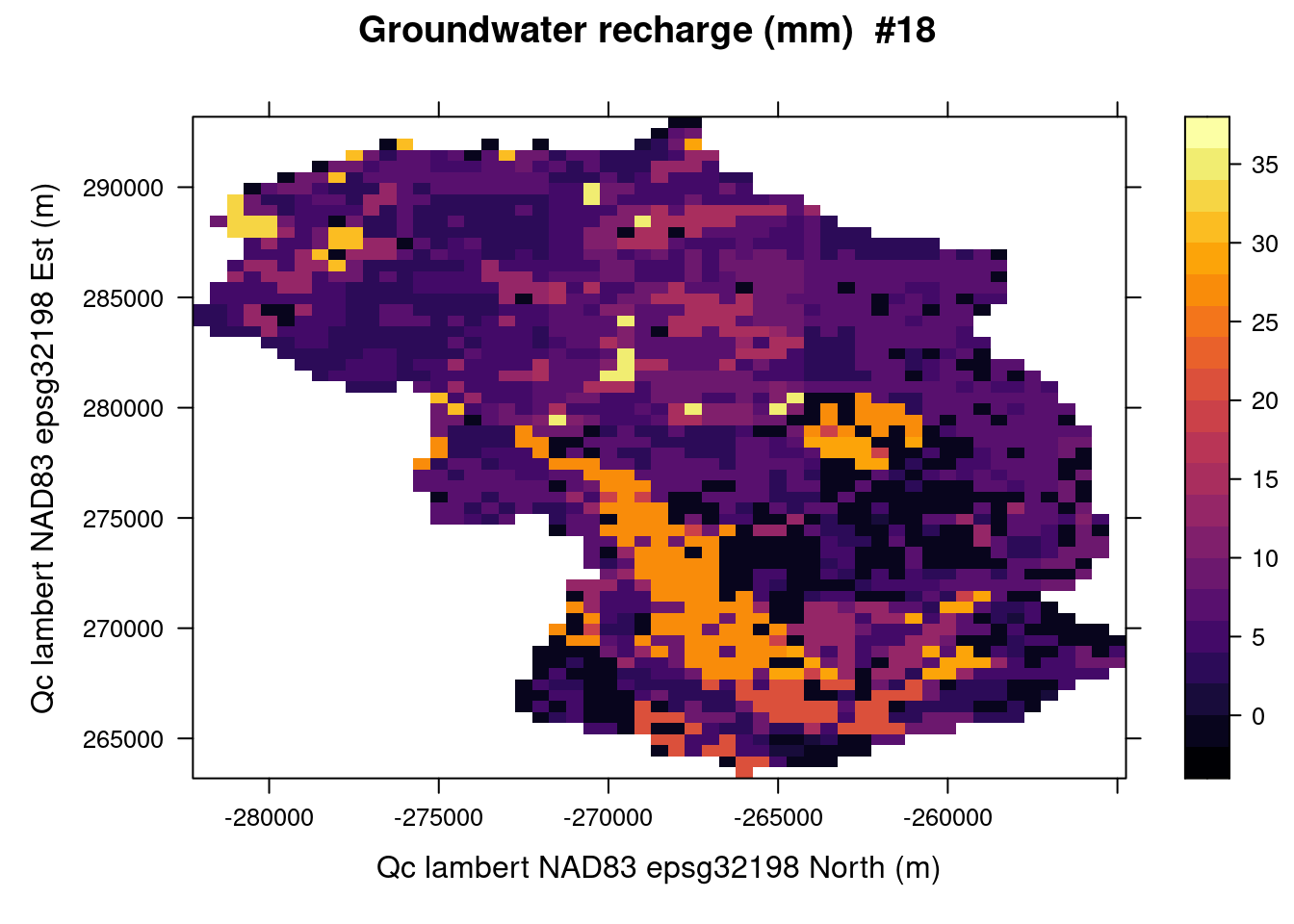
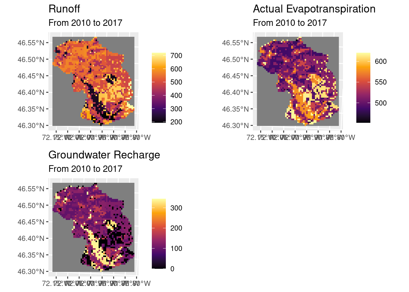
Visualize the saved raster files:
library(tidyterra)
library(terra)
library(ggplot2)
library(cowplot)
subtitle <- ifelse(simul_period[1] == simul_period[2],
  paste0("In ", simul_period[1]),
  paste0("From ", simul_period[1], " to ", simul_period[2])
)
runoff <- terra::rast(file.path(sim_dir, "interannual_runoff_NAD83.tif"))
runoffplot <- ggplot() +
  geom_spatraster(data = runoff) +
  scale_fill_viridis_c(option = "inferno") +
  labs(
    fill = "",
    title = "Runoff",
    subtitle = subtitle
  )
aet <- terra::rast(file.path(sim_dir, "interannual_aet_NAD83.tif"))
aetplot <- ggplot() +
  geom_spatraster(data = aet) +
  scale_fill_viridis_c(option = "inferno") +
  labs(
    fill = "",
    title = "Actual Evapotranspiration",
    subtitle = subtitle
  )
gwr <- terra::rast(file.path(sim_dir, "interannual_gwr_NAD83.tif"))
gwrplot <- ggplot() +
  geom_spatraster(data = gwr) +
  scale_fill_viridis_c(option = "inferno") +
  labs(
    fill = "",
    title = "Groundwater Recharge",
    subtitle = subtitle
  )
cowplot::plot_grid(runoffplot, aetplot, gwrplot)